GFD Lab XIV: Thermohaline Circulation of the ocean
Here we illustrate the dynamical principles that underlie the abyssal circulation of the ocean, driven by sinking of dense fluid formed by surface cooling at polar latitudes. As in Lab XIII we represent the sphericity of the Earth with a sloping false bottom. The sinking of water at polar latitudes is represented by a source of fluid in the top right-hand-corner of the tank.
We set a tank of water rotating at speed f = 2 (~ 10 rpm), as sketched in the diagram below. The square tank, of side 60 cm, whose bottom is inclined to the horizontal, is filled with water at constant temperature to a depth of 20 cm or so. The shallow end of the tank represents ‘North’, the deep end ‘South’, as in Lab XIII.
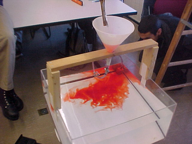
Dyed water at the same temperature is then slowly introduced in to the top right-hand-corner of the tank through a hose (fitted with a diffuser) at a rate 100ml/minute. The photograph on the right below shows the funnel device used to introduce the dyed (red) fluid. The funnel is in the rotating frame; a reservoir of dyed fluid stands on the top of ladder in the laboratory (non-rotating) frame.
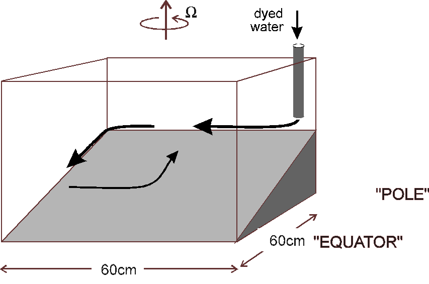
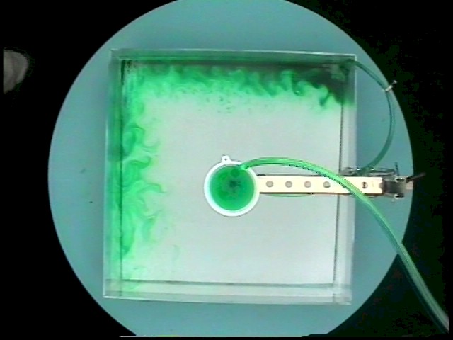
The rotating tank fills up with water in a manner that is very different from that in which a non-rotating tank would fill up. Instead of the dyed fluid ‘diffusing’ in to the interior, it runs along the northern boundary of the tank and feeds in to a ‘western’ boundary current, as sketched in the diagram above.
Have a look at the sequence of the pictures below illustrating how the tank fills up with water.
You can view a movie loop here.
Theory and interpretation
Let ‘h’ be the depth of the fluid, α the slope of the bottom, ‘L’ the side of the square tank and ‘S’ the rate at which water is introduced through the diffuser.
The free surface of the water rises at a rate given by:
![]()
Because the fluid is rotating and is in steady, slow, frictionless motion then, by the Taylor-Proudman theorem, columns must remain of constant length. Hence Taylor columns in the interior of the tank must move toward the shallow end of the tank to retain their length as the free surface rises. The northward speed at which they move is given by:
![]()
The general pattern of currents observed in the experiment is shown in the figure below.
It is useful to estimate typical interior speeds from the formulae above: typical experimental set-ups have
α = 0.2, L= 60 cm, Ω = 10 rpm and S=100ml/minute.
Finally, think about the relevance of the experiment to the thermohaline circulation of the ocean.
What do the parameters S, α, L and Ω correspond to oceanographically? Insert some oceanographic values for S, α, L and Ω, and hence estimate typical current speeds associated with thermohaline flow in the ocean.
Look at a simulation of CFC’s invading the ocean here.